Pivot Wizard

The Pivot Wizard generates pivot tables in your workbook from data model fields. You select the environment, data model, and fields you want to analyze, and the wizard creates a pivot table that you can then arrange by dragging fields into rows, columns, values, and filters. The pivot table updates automatically as you change the layout.

You can also apply filters and filter groups before creating the pivot to control which data is included, and configure options like automatic refresh and row limits.

When to create a pivot

• Summarize large datasets by aggregating data from a data model into a table with rows, columns, and calculated values.
• Analyze data across dimensions like product, region, customer, or time period by dragging fields into different areas.
• Filter data before building the pivot to limit the dataset to exactly what you need, rather than pivoting everything and filtering after.

Create a pivot table

1. Select an empty cell.
2. On the Analysis tab, select Pivot Wizard.
3. Select the environment and data Model.
4. Enter a name in the Pivot Name field.
5. On the Fields tab, search for or select the fields to include.
6. (Optional) Add filters or groups.
7. Click Create. The pivot table shows with the Pivot Table Fields.

Pivot properties

Property	What to configure
Environment	The environment to pull data from. If set to Current Environment, data is retrieved dynamically from whichever environment is active.
Data Model	The data model to use for the pivot.
Pivot Name	A name to identify this pivot in the workbook.

Select and configure fields

The Fields tab is where you choose which dimensions, descriptions, and measures to include in the pivot. Search for a field in the left panel, then drag it or double click it to add it to the center area.

• Group By determines whether this field is used to group rows. When off, it’s included in the results but doesn’t create groups.
• Order By controls how grouped data is sorted.
• Aggregation reduces the number of rows by applying an operation to the field before the pivot processes it. The pivot calculations are based on this aggregated result, not on raw data.

Example

Sales by product line with total revenue#

Total revenue by product line, sorted from highest to lowest.

Details

The pivot returns one row per product line, with net sales summed and sorted from highest to lowest.

Example

Unique customers and total sales by region#

Compare unique customers and revenue across regions.

Details

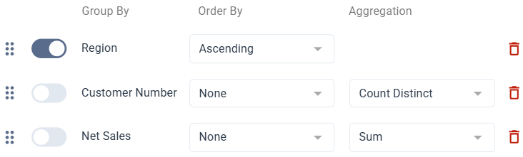
The pivot returns one row per region, showing the number of unique customers and total net sales for each.

Options

Option	What it does
Refresh on Open	Automatically refreshes the pivot when the workbook is opened.
Automatic Refresh	Automatically refreshes the pivot when a related filter value changes.
Top X	Limits the number of rows returned by the pivot.
Worksheet	Controls where the pivot is placed: Existing Worksheet inserts the pivot at the specified location. New Worksheet creates a new sheet and inserts the pivot at the top left cell.
Location	The cell where the pivot is inserted. Shown when using an existing worksheet.

Add filters to a pivot

Filters narrow what data the pivot includes. You can add individual filters or filter groups, and combine them with And / Or logic. For each filter, you select a field, an operator, and a value.

• Individual filters target a single condition.
• Groups wrap multiple filters together so they are evaluated as one unit.

Values can be entered manually or by referencing a cell. You can also search for a specific value using the prompt icon next to a filter. Select a filter method from the prompt to search, or use wildcards for more precise matching.

Enter filter values

Each filter value can be entered as a text string or as a cell reference. The behavior depends on how the value field is configured.

Mode	How it works	How to set it
Cell reference	The value is pulled dynamically from a cell in your sheet. The pivot updates when the cell value changes.	Select the underscore in the value field, then select the cell in your sheet.
Text string	The value is typed directly and stays fixed regardless of what's in your sheet.	Select the A icon next to the value field. When active, the icon turns blue.

note

If you use the prompt to select a value, it is automatically set as a text string.

Search values with wildcards

Wildcards and expressions apply only to text values, not numbers. To use them, select the prompt icon next to a filter and choose wildcards from the filter method. These expressions work with the Equal, Not Equal, In List, and Not In List operators.

Supported wildcards

• ? matches exactly one character
• * matches one or more characters
• ! excludes characters or ranges
• ; separates multiple values
• & combines conditions
• [a:b] defines a range between two values
• "..." treats special characters as literal text

Example	What it matches
4000	Matches exactly 4000.
4000;5000;6000	Matches 4000, 5000, or 6000.
4*	Matches any value starting with 4.
4???	Matches values starting with 4 with exactly four characters.
A*&*Z	Matches values that start with A and end with Z.
[4000:4999]	Matches values between 4000 and 4999.
[A*:F*]	Matches values from A through F using prefix matching.
!4000	Excludes 4000.
!4*	Excludes values starting with 4.
!4???	Excludes values starting with 4 with exactly four characters.
[10000:10200]!10100	Matches values between 10000 and 10200, but excludes 10100.
!1000;2000;7000	Excludes 1000, 2000, and 7000.
"10:00"	Matches the literal value 10:00 (: is not treated as a range operator here).
[4???:5???]	ERROR ? inside a range bound is not supported.
[A*B:C] or [**:C]	ERROR * in the middle of a range bound or multiple * in a range bound are not supported.

Arrange fields in the pivot table

After creating a pivot, the Pivot Table Fields panel opens on the right. This is where you arrange how data appears in the pivot table by dragging fields into the areas below.

Areas

Areas

Area	What it does
Filters	Fields placed here act as top level filters for the entire pivot table.
Columns	Fields placed here become the column headers of the pivot table.
Rows	Fields placed here become the row labels of the pivot table.
Values	Numeric or calculated fields placed here are aggregated and displayed as the pivot table values.

Field selection

Field selection

Select fields from the data model using checkboxes. Fields are automatically placed based on their data type: numeric fields go to Values, while text or categorical fields go to Rows. You can drag fields to other areas as needed.

Additional options

Additional options

Option	What it does
Defer Layout Update	Pauses pivot updates while you rearrange fields. Select Update to apply all changes at once.
Views	Switch between saved field layouts or select from predefined views of the pivot table.

Edit a pivot table

1. Select a cell inside the pivot table.
2. On the Analysis tab, select Pivot Wizard.
3. Make your changes.
4. Select Save.

Refresh a pivot table

Refreshing updates the pivot table with the latest data from the data source.

1. On the Toolbar panel, select Refresh.
2. Make sure the Pivots toggle is on.
3. Select Entire Workbook to refresh all pivot tables, or Current Sheet to refresh only the active sheet.